
Thomas F. Collura, Ph.D., MSMHC, QEEG-D, BCN, LPCC-S
(Note on construction: this post was drafted with Claude.ai under the author’s direction, from the author’s earlier posts on sLORETA relative power and on homomorphic deconvolution, and from the published preprint discussed below. The technical content and the interpretation are the author’s.)
“Activity equals results. If you want to increase your success, Increase your activity.”
— Brian Tracy
Where we left off
In Part I I described how sLORETA and its relatives compute the current-source density in a small volume of brain — a “region” — from the 19 channels of scalp EEG, and I argued that the most useful thing we can ask of such a region is not how much current it is producing, but how it is distributing that current across the frequency bands — that is, its relative power. Absolute power tells us how hard a region is working. Relative power tells us what it is working on. The claim was that this answers a different and more interesting question: not “what is going on?” but “what is important right now?”
I want to extend that argument, because two developments have made it considerably sharper than it was when I first made it. The first is a modeling result published this summer by Giulio Ruffini’s group, which gives the cortical column a precise identity as a tuned receiver. The second is our own work on homomorphic deconvolution of the EEG using ICA, which has convinced me that the generators we are imaging are better described as event generators than as frequency generators. Those two things sound as though they should be in tension. They are not. Taken together, they explain why relative power is the right readout — and they tell us what it is actually a picture of.
One region, more than one job
In Part I, almost in passing, I wrote that the cortical layers are complex, and allow one region to do more than one thing — either in sequence, or at once — and that this is the basis of the different EEG bands. By knowing which are the dominant bands in a given region, we know what the region is doing, and which networks it is binding into at their characteristic frequency, such as alpha for the default mode network (DMN).
That remark deserves more weight than I originally gave it, because the anatomy behind it is not incidental — it is the whole mechanism.
A cortical column is not a homogeneous lump of tissue that happens to oscillate. It is a laminated structure in which each layer has its own cell populations, its own interneuron types, its own inputs, and its own outputs. Thalamic input arrives in the middle layers. Superficial layers project forward, to the next area up the hierarchy. Deep layers project back, down the hierarchy, and out to subcortical targets. The inhibitory cells differ layer by layer: fast, perisomatic parvalbumin (PV) interneurons dominate the superficial fast circuitry; slower, dendrite-targeting somatostatin (SST) interneurons figure in the deeper loops. And because the frequency of a neural oscillation is set largely by the time constants of the inhibition in the loop that produces it, different layers, with different interneurons in different loops, produce different frequencies.
So each layer may participate in its own connections and its own rhythms. The consequence is worth stating plainly, because it is easy to lose behind the tidy colors of a band map:
Each cortical column is a complex, multifrequency generator. It is not an alpha generator that sometimes does something else. It is a stack of coupled loops, several of which can ring at their own rates, at the same time, at different depths, doing different jobs.
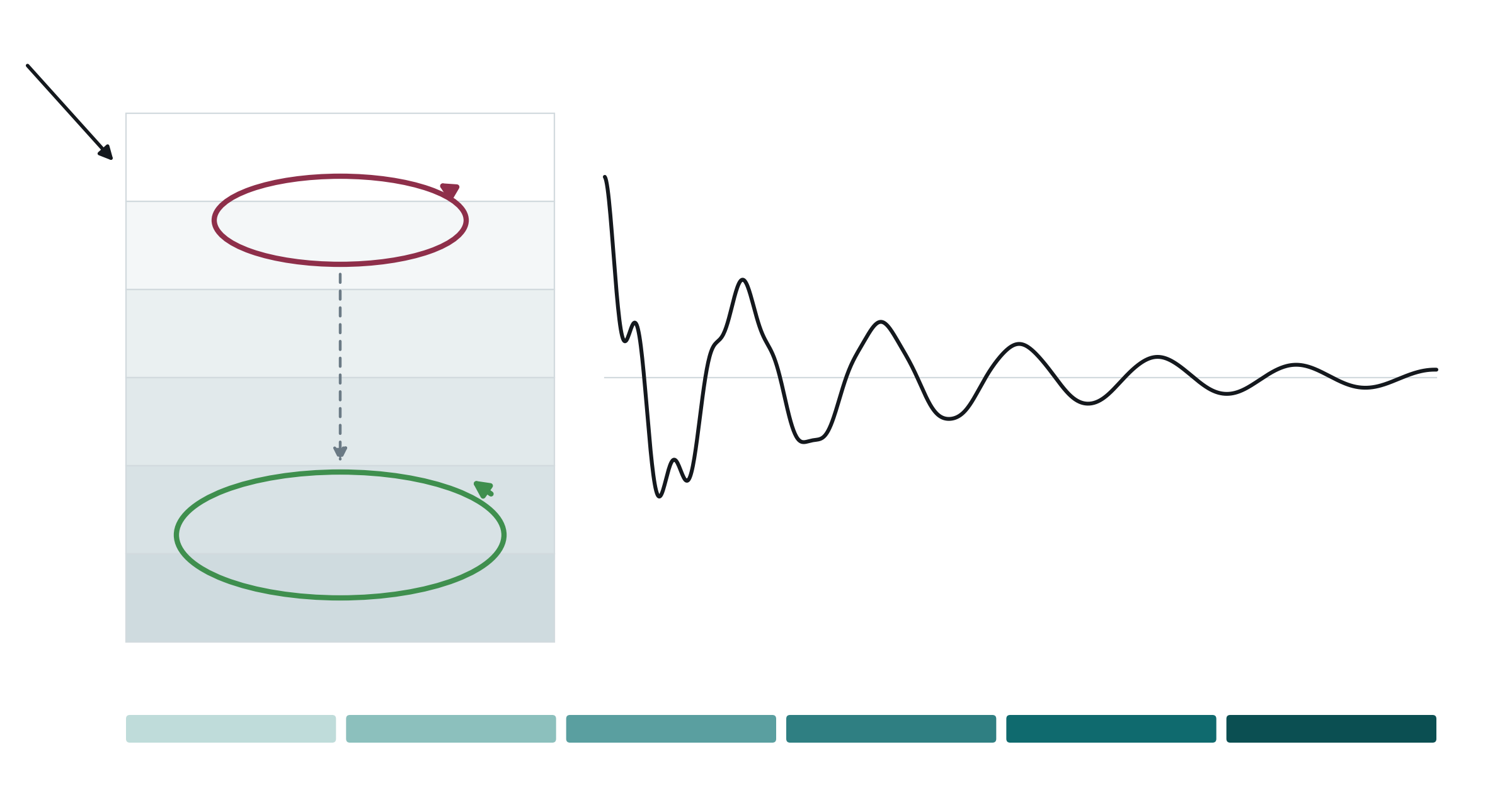
If that is what a column is, then the question “what frequency is this region?” is malformed. The right question is the relative-power question: of everything this column is currently doing, how is it dividing its effort?
The column as a tuned receiver
The modeling result that sharpened this for me comes from an unexpected direction — the physics of brain stimulation rather than the analysis of brain signals.
Ruffini and colleagues (2026) set out to solve a puzzle in temporal-interference (TI) stimulation. TI delivers two high-frequency currents whose amplitudes beat at a low difference frequency, and the brain appears to respond to the beat. But an amplitude-modulated field carries no power at the beat frequency. There is nothing at 10 Hz in a 10 Hz-beating pair of 2 kHz carriers, in the same sense that there is nothing at 1 kHz in an AM radio broadcast until something in the receiver demodulates it. Recovering the beat requires a nonlinearity, and the field has for years looked for that nonlinearity in single-cell ion channels.
Their answer is that the recovery, and more importantly its tuning, are properties of the population, not the single cell. In a neural mass — the roughly 10⁴-neuron unit that actually generates the EEG we record — two things happen in sequence:
- The firing-rate nonlinearity acts as a square-law detector. The sigmoid relating a population’s mean membrane potential to its mean firing rate is curved, and a curved transfer function mixes frequencies. Squaring an amplitude-modulated carrier produces a term at the modulation frequency. The envelope is recovered. This is the detector stage, and it is inherited from the single neuron.
- The recurrent synaptic network, poised near a Hopf bifurcation, resonantly amplifies the recovered rhythm at its own natural frequency. This is the tuned tank, and it is emergent — a property of the network’s connectivity and of how close the network sits to its own instability, not of any cell in it.
The authors are explicit about the analogy, and it is exact rather than decorative: the stages “map onto the RF front end, square-law/diode detector, RLC tank, and audio output of a classic AM receiver.” Their conclusion — “the cortical column behaves as a tuned AM radio receiver” — is the sentence I would put on the wall.
INSERT IMAGE HERE: fig-receiver.png (from the art folder) — then delete this line
The two-band column, read as a receiver (stages after Ruffini et al., 2026, §2.1 and §4.5). The superficial fast loop must itself be excited before it can pass a demodulated envelope to the deep slow loop — a receiver with stages, not a bank of independent filters. What comes out is a change in timing while the mean firing rate stays flat.
Three details of their laminar model matter for us.
A column has more than one native resonance. Their laminar neural mass model (LaNMM) couples a deep, Jansen–Rit-like subcircuit — pyramidal cells with spiny-stellate and SST interneurons, intrinsic rhythm alpha, 10 Hz — to a superficial PING-like subcircuit — pyramidal cells with PV interneurons, intrinsic rhythm gamma, 40 Hz. One column, two native resonances, at two depths, built out of two different interneuron populations. That is the multifrequency generator, written down as equations.
The two resonances are cascaded, not parallel. When the modulated input is delivered to the superficial fast loop, a strong response in the deep slow loop requires a double resonance: the carrier near the superficial gamma, and the beat near the deep alpha. As they put it, “the fast loop acts as a tuned ‘RF front end’ that must itself be excited before it can pass a demodulated envelope” to the deep loop. A column is not a bank of independent filters. It is a receiver with stages.
The tuning is a state variable, not fixed hardware. The sharpness and the gain of the resonance are “set by how near the network sits to criticality, and tunable by its own connectivity.” Move the operating point — with neuromodulation, with arousal, with task — and the same anatomy becomes a differently tuned receiver. Their clinical inference concerns stimulation: “TI efficacy should be as much a property of the brain as of the device.”
Ours is about measurement. If a column’s tuning is a state variable, then it is something we can image. Relative power is the picture of where a column’s gain currently sits.
Why relative power is the right readout
The core observation of Part I was that, once volume conduction is taken out and we are looking at one spot in the brain rather than a scalp mixture, any given area of cortex has limited freedom to do different things at once, and so will tend to be busy with one thing at a time as the brain moves through its microstates and processing sequences.
The tuned-receiver picture tells us why that is true, and in what sense. A near-critical resonator has high gain in a narrow band; if the operating point favors one of a column’s resonances, that resonance takes a disproportionate share of the energy. Being “busy with one thing” is not a statement about the column’s wiring. It is a statement about its momentary allocation of gain among resonances it possesses permanently.
This also rehabilitates the standard objection to relative power. Every QEEG course teaches, correctly, that relative power couples the bands: they sum to 100%, so a relative-power excess in one band may reflect a deficit elsewhere, and an apparent finding may live in a different band than the one it is painted in. That is a genuine hazard when you are trying to read relative power as a proxy for absolute magnitude. But when the quantity of interest is the allocation — when the question is which resonance is currently being favored — the coupling is not an artifact. It is the measurement. A tuned circuit that puts more of its energy into 10 Hz has less to put anywhere else, and saying so is the whole point.
Report both, as always. Absolute power tells you how hard the column was struck. Relative power tells you how well, and at what frequency, it rang.
But the generators are not oscillators
Here is where our own ICA work complicates the picture in a productive way.
We have implemented a system that performs homomorphic deconvolution of resting EEG, using a built-in ICA, frequency-domain averaging, sLORETA, and source localization to deconvolve EEG rhythms into individual sources and patterns. ICA converts 19 channels of EEG into 19 components, removing the effects of volume conduction and converting the mixed signals from the scalp into a set of estimated sources. Each source has its own scalp distribution (the mixing matrix), its own time series, its own sLORETA localization — and its own complete frequency spectrum.
That last point is the one that matters here, and it surprised us when we first looked at the Brain Panel decompositions carefully. These are not narrow-band oscillators. A well-localized dipolar source — a component whose scalp map is clean, whose sLORETA solution is compact, and whose classification is unambiguous — routinely shows a complex, broad spectrum. Component 3 in one of our resting records arises from the parahippocampal gyrus and “contains a wide range of frequencies encompassing essentially the entire range of EEG frequencies.”
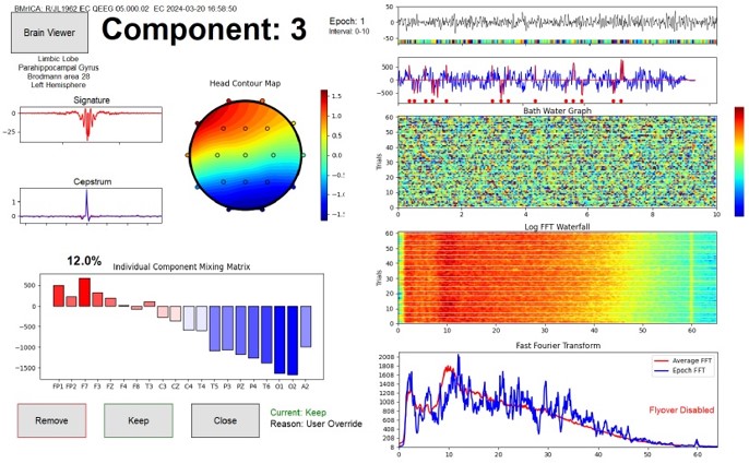

Component 3 from a resting, eyes-closed record, as the BrainAvatar ICA panel shows it: a compact left parahippocampal source (Brodmann area 28), with its extracted signature, scalp map, mixing matrix and time course — and an averaged spectrum that runs from the low end of the EEG to past 40 Hz. Below, its sLORETA localization. One clean source; no single frequency.
So localization does not buy you monochromaticity. Removing volume conduction does not reduce a source to a tone. What each component has instead is a signature — a fingerprint, a characteristic morphology — which the deconvolution recovers by averaging in the frequency domain and inverting, and which we can then find again in the raw component signal by template matching.
The framing that follows from this is the one I now prefer:
The EEG does not consist of a lot of free-running frequencies. It consists of things that happen at particular times. If the brain were a bell being rung, the question is what the response to one ring looks like, and what the pattern of striking is over time. These signatures occur intermittently — more of a series of chirps than a frequency.
Which is to say: the sources we image are event generators, not frequency generators. They are not oscillators that we sample; they are structures that get struck, and ring.
Reconciling the two pictures: the bell and the tank
Set those two results side by side and the apparent contradiction dissolves immediately.
Ruffini’s column is a tuned tank. Our ICA component is a bell being struck. Those are the same object described from its two ends. A resonator’s ring is determined by the resonator; the timing of the rings is determined by the events that excite it. Strike a multi-resonant structure with a brief, broadband event and what comes out is a complex waveform whose spectrum reflects all the resonances the event happened to excite, weighted by how near each one sits to criticality at that moment. Do it intermittently, at irregular intervals, and the averaged spectrum of the resulting time series is broad — exactly what the component spectra show.
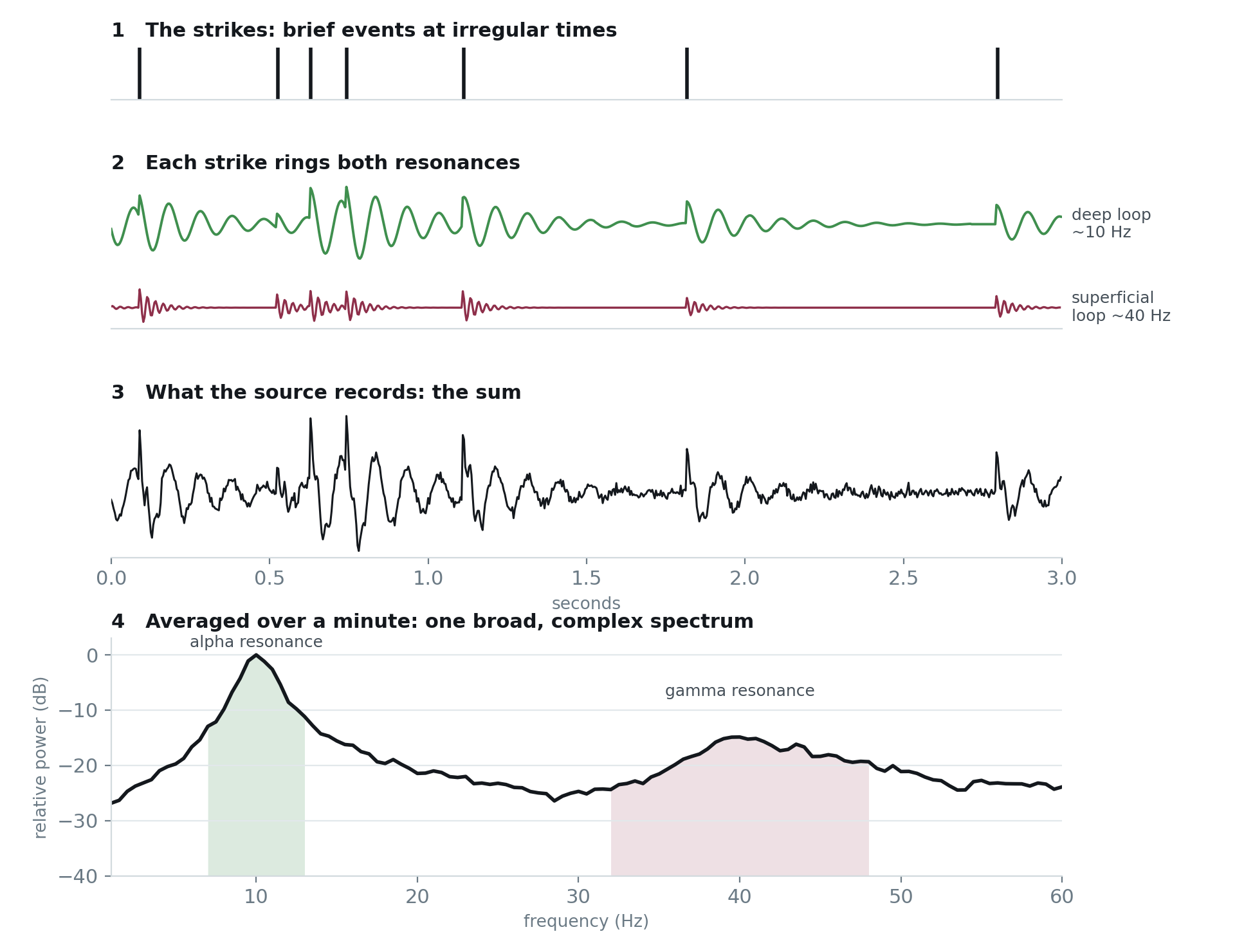
The bell and the tank, simulated. (1) Brief events arrive at irregular times. (2) Each one rings both of a column’s resonances — a slow, lightly damped deep loop near 10 Hz and a fast, quickly damped superficial loop near 40 Hz. (3) The source records their sum, which looks like anything but a sine wave. (4) Averaged over a minute, the spectrum is broad and complex, with the two resonances standing up out of it. An illustration built from two damped oscillators, not a recording.
A complex component spectrum is therefore not evidence against tuning. It is what tuning looks like when the excitation is transient rather than sustained.
And the two accounts converge on the same methodological punchline. One of the more striking results in the Ruffini paper is that the near-Hopf resonance “amplifies oscillatory timing far more than mean rate” — it locks spike timing without changing firing rate, which is precisely what has been observed in the primate brain in vivo (Vieira, Krause, & Pack, 2024). Timing, not rate. Our own conclusion from the deconvolution work was events, not frequencies. Those are the same claim at two scales — one in a mean-field model of a column, one in the decomposed surface EEG of a person sitting in a chair. When two independent lines of work arrive at the same statement from opposite directions, it is usually worth taking seriously.
Layers, not just regions
If the frequencies in a column are produced by loops at different depths, then a band-dominance map carries more information than “this region is busy.” It carries a hypothesis about which laminar loop is doing the work.
In the laminar model, the slow loop is the deep one and the fast loop is the superficial one. Superficial layers are the feedforward, next-area-up pathway; deep layers are the feedback and output pathway. In the cross-frequency-coupling account of predictive coding that the same group has developed (Ruffini et al., 2025), that division of labor is the substance of the computation: the deep, slow activity carries the prediction, the superficial, fast activity carries what the prediction failed to explain, and the coupling between them — the sigmoid demodulating one against the other — is the comparison.
Read through that lens, an alpha-dominant voxel and a gamma-dominant voxel are not just two different colors on a map. They are candidate signatures of two different directions of traffic through the same piece of cortex.
A caution is essential here, and I want to state it rather than bury it. LORETA-family methods do not resolve cortical layers. A voxel’s current-source density is a summed dipolar quantity to which every layer contributes. The inference above is about which laminar loop appears to dominate that sum, and it is a hypothesis suggested by a model — a well-constructed model, in a preprint, tested against stimulation data rather than against QEEG. It is not a measurement of laminar activity, and nobody should report it as one. What it does is give the band-dominance map a mechanism to point at, which is a considerable improvement over pointing at nothing.
Why the bands sit where they do
One more piece from the same line of work is worth flagging, because it speaks to something the field usually treats as historical accident.
The Hierarchical Amplitude Modulation framework (Ruffini, 2025) generalizes the demodulation idea to nested envelopes with constant-Q, logarithmically spaced bands — envelopes of envelopes — and proposes this as a candidate origin of the 1/f spectrum, again through the quadratic cross-term in the sigmoid. Readers of this blog will recognize the shape of that claim: it is close kin to the binary frequency hierarchy and golden-mean band separation that Bill Brubaker and I discussed in connection with David Cantor’s relational-architecture preprint, and to Klimesch’s account of the band center frequencies as a scaled hierarchy rather than a set of conventions.
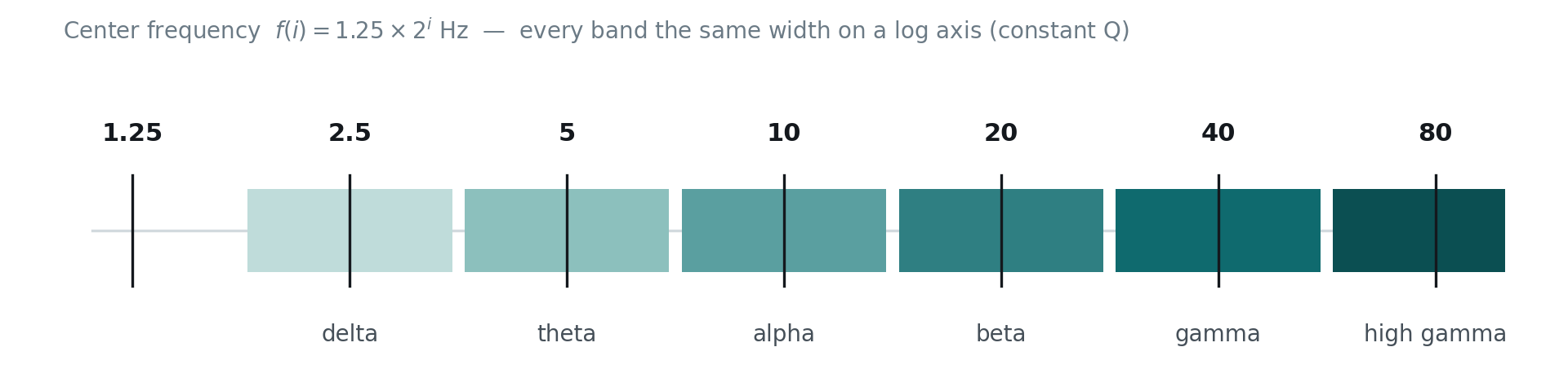
The constant-Q ladder: center frequencies f(i) = 1.25 × 2ⁱ Hz, after Klimesch (2018) and as discussed in Cantor (2025). On a logarithmic axis every band is the same width — the ratio of bandwidth to center frequency never changes.
If the bands really are a constant-Q ladder, then the relative-power pie is not an arbitrary carving of the spectrum. Its slices are the architecture’s own coordinates, and asking how a column divides its energy among them is asking a question the structure is built to answer.
What this buys the clinician
Part I showed what the sLORETA and eLORETA relative-power maps look like in BrainAvatar — regions lighting up only when a significant fraction of their energy sits in the band of interest, networks appearing and disappearing with each use, the isofield rendering and the region-and-hub text display — and that they serve neurofeedback as well as assessment and progress tracking.
What the tuned-receiver picture adds is a reason to treat those maps as tuning maps, and two practical consequences.
First, on choosing a frequency. The result that a forced response is “largest when the beat matches a region’s intrinsic rhythm,” with a gain that depends on the brain’s current state, applies to any attempt to drive a network — stimulation, photic entrainment, or the much gentler push of a reward contingency. Feedback lands where gain already is. A relative-power map is an estimate of where the gain currently is, and that is usable information at protocol time: train the band a region is demonstrably able to favor, or if the goal is to shift the allocation, know that you are working against a tuned circuit and not merely against a number.
Second, on what to reward. If the generators are event generators, then power training is training a proxy. Knowing the shape of each event lets us do real-time cross-correlation and reward occurrences of the transient itself — rewarding a brain event rather than a frequency. That work is under way, and patents have been applied for. Relative power and event-based training are not competitors: the first tells you which of a column’s resonances is currently favored, the second lets you reinforce the actual striking of it.
What is not settled
It is worth being clear about the status of all this. The tuned-receiver mechanism is a modeling result in a preprint, demonstrated in a heuristic column, a laminar two-band column, an exact next-generation mean field, and a spiking network — internally consistent and tested against the stimulation literature, but a model. The laminar reading of band dominance is an inference, for the reasons given above. Instantaneous relative power computed from short epochs is noisy, and the shorter the window the more it wanders. And relative power remains a ratio: it should be read next to absolute power, not instead of it.
None of that touches the core observation, which is an empirical one and available to anyone with the software in front of them. A localized source has a complex spectrum. A column has more than one resonance. And the fraction of its energy sitting in each band changes from moment to moment in a way that tracks what the brain is doing.
sLORETA and eLORETA relative power open up new possibilities for QEEG and neurofeedback. What has changed since I last wrote about it is that we now have a mechanism to attach the maps to: not a set of independent oscillators to be counted, but a stack of tuned circuits being struck by events, with the tuning itself as the thing that varies — and with relative power as the instrument that reads it.
BrainAvatar continues to lead the way, implementing new and effective methods, building on what has already been learned and moving toward what is yet to be learned.
“New information makes new and fresh ideas possible.”
— Zig Ziglar
References
Cantor, D. S. (2025). Relational geometry and frequency architecture: Patterns of order across brain, body, and cosmos. Preprint. (Discussed in Brubaker & Collura, “Cantor’s Relational Architecture and Brain Oscillatory Tensegrity,” BrainMaster Technologies — Perspectives in Neurofeedback, 2026. https://brainmaster.com/cantors-relational-architecture-and-brain-oscillatory-tensegrity/)
Collura, T. F. (2025). Advances in EEG analysis — Homomorphic deconvolution of EEG using ICA and sLORETA. BrainMaster Technologies — Perspectives in Neurofeedback. https://brainmaster.com/advances-in-eeg-analysis-homomorphic-deconvolution/
Collura, T. F. (2025). Probing the priorities of the brain: sLORETA. BrainMaster Technologies — Perspectives in Neurofeedback. https://brainmaster.com/probing-the-priorities-of-the-brain-sloreta/
Grossman, N., Bono, D., Dedic, N., et al. (2017). Noninvasive deep brain stimulation via temporally interfering electric fields. Cell, 169(6), 1029–1041.e16.
Klimesch, W. (2018). The frequency architecture of brain and brain body oscillations: An analysis. European Journal of Neuroscience, 48(7), 2431–2453.
Ruffini, G. (2025). Neural encoding through hierarchical amplitude modulation. bioRxiv 2025.11.03.686310.
Ruffini, G., Lopez-Sola, E., Palma, R., Sanchez-Todo, R., Vohryzek, J., Castaldo, F., & Friston, K. (2026). Cross-frequency coupling as a neural substrate for prediction error evaluation: A laminar neural mass modeling approach. Neural Computation, 38(8), 1299–1343. https://doi.org/10.1162/neco.a.1537
Ruffini, G., Mercadal, B., Just, A., de Palma Aristides, R., Castaldo, F., Canals, S., & Mirasso, C. (2026). The cortical column as a tuned receiver: A network mechanism for temporal-interference stimulation (Version 0.11.0). Zenodo. https://doi.org/10.5281/zenodo.21305555 (quotations are from this version; the latest version is always at https://doi.org/10.5281/zenodo.21009618)
Vieira, P. G., Krause, M. R., & Pack, C. C. (2024). Temporal interference stimulation disrupts spike timing in the primate brain. Nature Communications, 15, 4558.
Tom Collura Ph.D., MSMHC, QEEG-D, BCN, NCC, LPCC-S, Founder BrainMaster Technologies, Inc.