We have implemented a system that performs homomorphic deconvolution of resting EEG samples, using a built-in ICA, frequency-domain averaging, sLORETA, and source localization to deconvolve EEG rhythms into individual sources and patterns. The signature captures the morphology of one “event” being produced by that brain source. The question being asked is, if the brain were a bell being rung, what is the response of one ring, and what is the pattern of the bell being struck as a pattern in time. Thus, the EEG does not consist of a lot of free-running frequencies, it consists of things that happen at particular times.
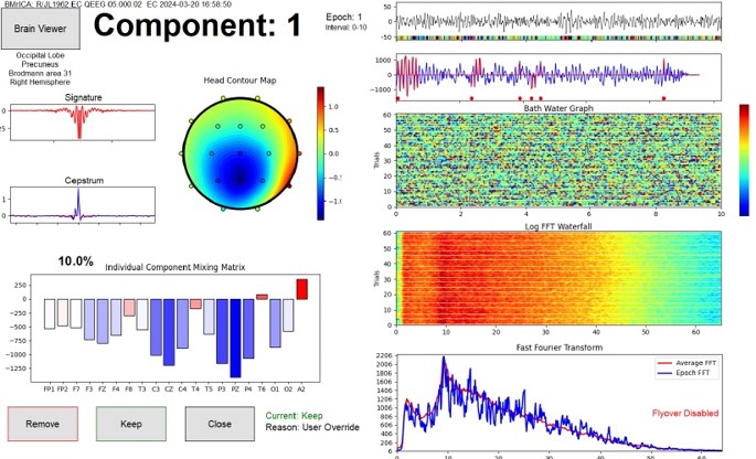
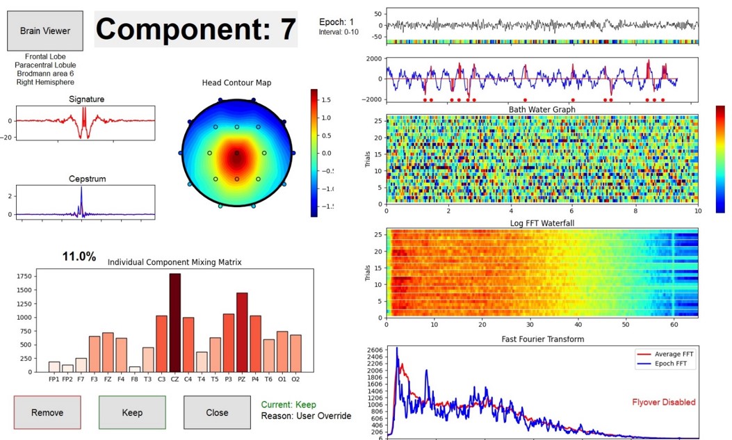
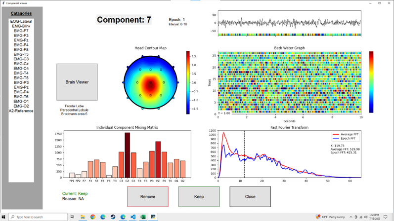
Components 1 and 7 show a posterior dominant rhythms, coming from different sources, and with slightly different spectral distributions. These are individual characteristic for that individual. We are investigating if these are reliably repeatable observations.
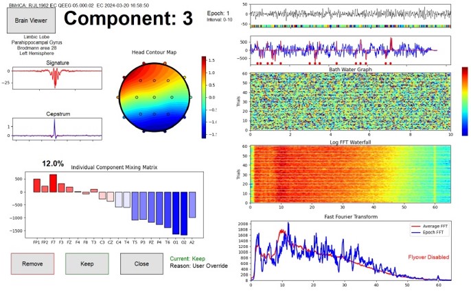
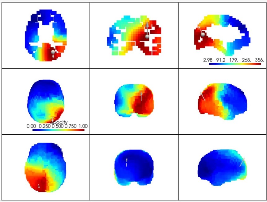
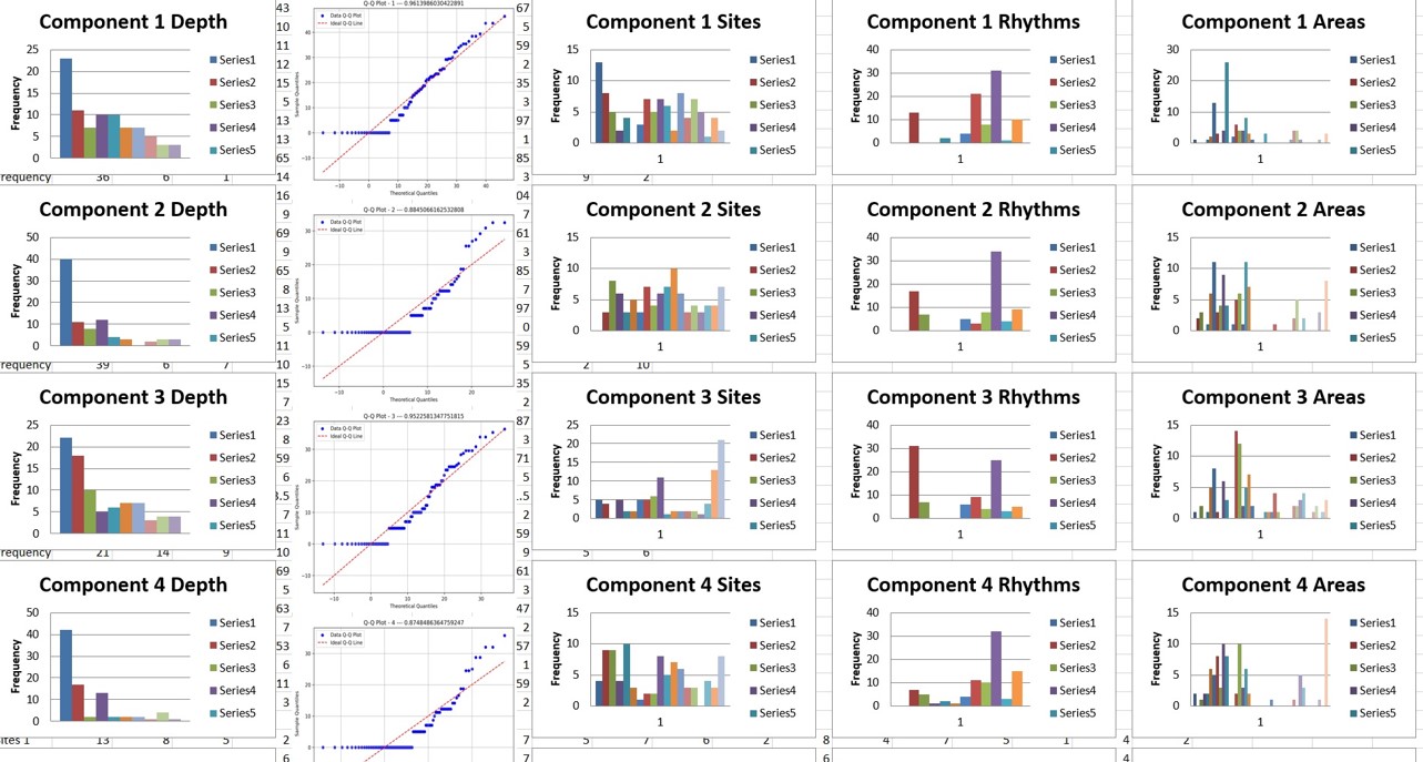
Component 3 is a mixed rhythm arising from the parahippocampal gyrus. It contains wide range of frequencies encompassing essentially the entire range of EEG frequenci

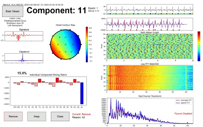
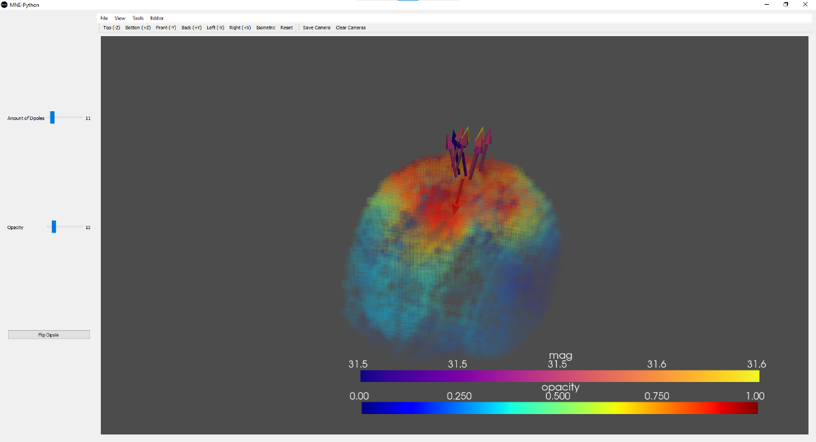
Component is 11 is EKG (electrocardiogram) artifact that is found to be maximum at A2. The method correctly identifies the signature, with the distinct appearance of a P-QRS-T wave morphology, confirming that this method is faithful to signal morphology. It also accurately poinpoints the heart beats using the template matching method, confirming the accuracy of this method as well. HRV statistics can be computed from this data. The source localization puts the source at the base of the neck, which is where the field actually appears to arise from, as volume conduction.
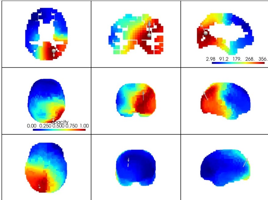
The timing statistics for these components is revealed in the points depicted on the example 10-second time-series plot. This plot is created by using a template-matching method that finds occurrences of the signature in the raw component signal across time.
The ICA (Independent Component Analysis) produces a set of individual components that are mathematically produced using an iterative procedure.. ICA is essential to this method, as it first converts the 19 channels of EEG into 19 components, which are signals that are distributed across the channels in a simple linear relationship. Thus, ICA removes the effects of volume conduction, and converts the mixed signals from the scalp into a set of estimated sources. Each source has a complete frequency spectrum. Sources should not be confused with channels, or with frequencies. Each source has its own amplitude for every channel (shown in the mixing matrix), and its own time series that runs through all channels, across the entire sample.
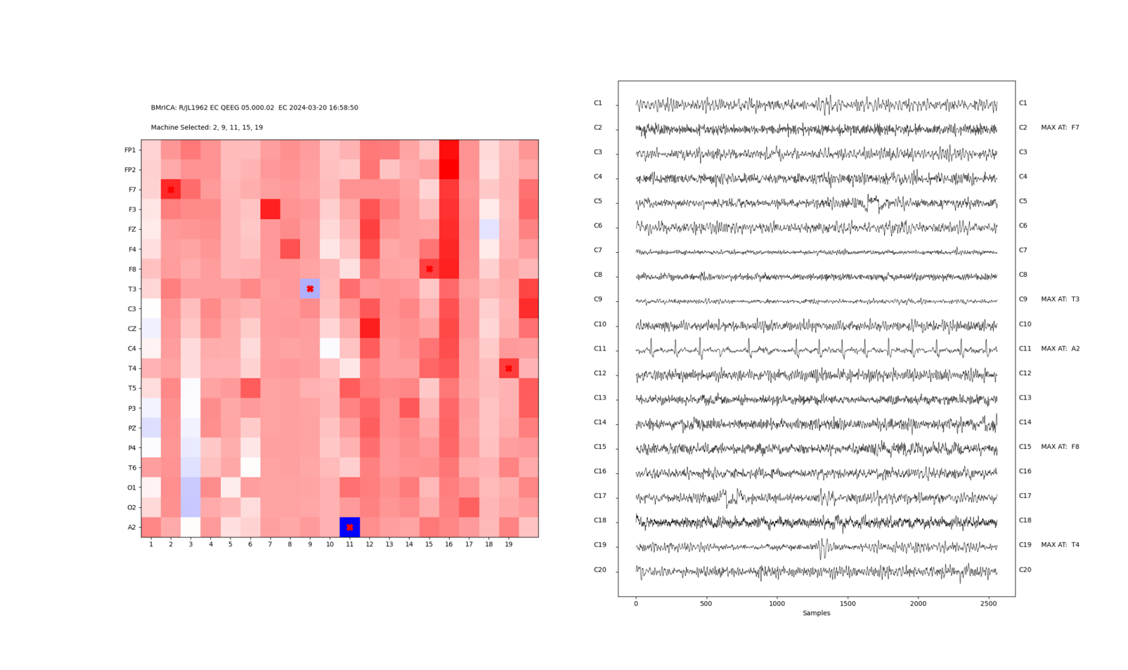
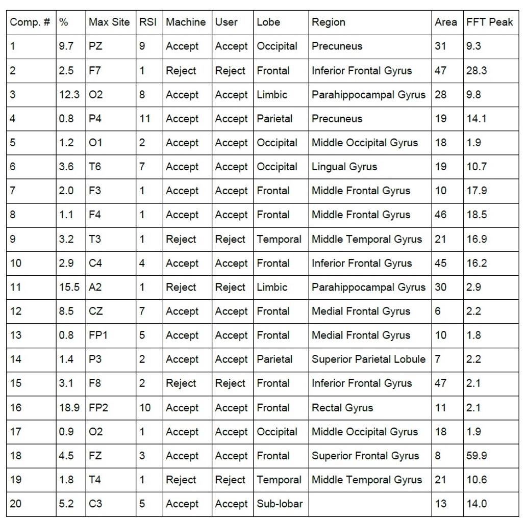
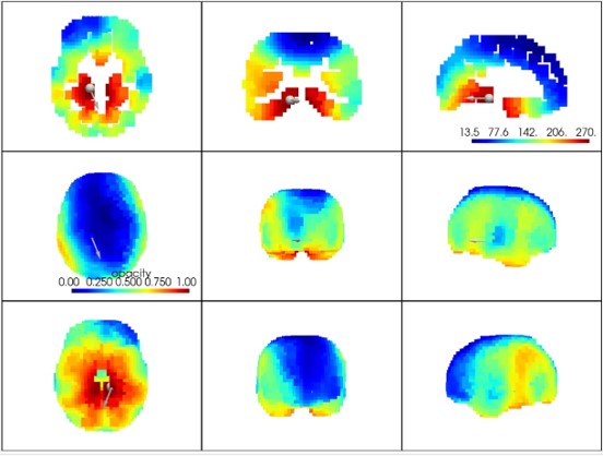
The list of components reflects important characteristics including the percentage of total EEG energy that is contained in the component, the surface site at which it is maximum, the machine and user decisions whether to accept the component for further processing, the sLORETA localized lobe, brain region, Brodmann area, and FFT peak energy. These allow us to classify components in categories such as artifact, posterior dominant rhythm (PDR), midline theta, frontal sources, and other classifications
This process does not use z-scores to create the localization or images. All data is processed as raw EEG, and no database is used in these computations. Is is posslble to create z-scores from this data, leading to a new kind of databse.
Rather than analyzing the EEG using strictly Fourier methods, which reduces the signal to a set of frequencies, this method takes advantage of ICA as a reverse source localization method which removes volume conduction. We think of the EEG as a series of events, not a simple vibration. Each component has a mixture of frequencies, and its own fingerprint or “signature.” These signatures are thought to occur in the EEG on an intermittent basis, providing more of a series of chirps than a frequency.
The viewing an analysis tools include an EEG viewer displaying the 10-second epochs, an individual FFT and averaged FFT graph, a “bathwater” graph of the component amplitudes color-coded across time for all epochs, and inverse of the averaged FFT, and the “periodigram” of the periods that the component is present in the original signal. When constructing a database, the statistics of this gating function become one set of metrics that can be characterized in a typical database.
We are creating a database of these results by classifying each component by type (e.g. PDR, midline theta, etc) and recording their occurrence in each EEG. Some EEG’s may have one PDR generator, while others may have two or more independent generators. These produce individual differences in EEG. The components provide the basis for a new type of database. This will contain data such as the depth of each component, its surface locations, frequency content, sLORETA location, classification, time statistics, and other information, so that each component source can be classified and rated in comparison to data obtained from hundreds of EEG recordings.
The database being constructed include classification for each component for each individual, peak frequencies, sLORETA depth, and statistics describing the time behavior of each component. This creates a new type of metric analysis that reflects underlying stable generators and time behavior in an individualized basis.
This provides the further possibility of creating neurofeedback based upon the template matching. Knowing the shape of each event, we can do real-time cross-correlation and reward occurrences of each transient, not just rewarding a “frequency”
This paves the way to a future in which EEG Biofeedback is based on actual brain events and timing, going beyond conventional power training, and moving into a world in which specific and individualized brain activity can be imaged, trained, and used in the application of brain plasticity and self-regulation.
Patents applied for.